Shadow prices

A single-phase solution returns, alongside the optimal controls and states, an estimate of the costate \(\lambda(t)\) of each state and the Hamiltonian \(H\). This page explains what these quantities mean, how to read them, and how to check them.

What they are

For an optimal-control problem with running payoff \(L\), dynamics \(\dot x = f(x,u,t)\), and terminal payoff \(M\), Pontryagin's maximum principle introduces one costate \(\lambda_i(t)\) per state and the Hamiltonian

\[ H = L(x,u,t) + \lambda^\top f(x,u,t). \]

Along a smooth optimum, the costate of state \(i\) equals the sensitivity of the optimal objective to that state,

\[ \lambda_i(t) = \frac{\partial J^*}{\partial x_i(t)}, \]

that is, the change in \(J^*\) per extra unit of state \(i\) at time \(t\), with the rest of the trajectory re-optimized. In economics and ecology this quantity is called a shadow price: the marginal value of a pool. Optimal rates change through time because these values change as pools are depleted, replenished, or approach the end of the period.

eco_opt does not derive costate equations. It recovers \(\lambda\) from the multipliers of the collocation equations of the discretized problem, a standard property of direct collocation (Benson et al., 2006; Garg et al., 2010).

Getting them

lam = sol.costate          # (N*d, nx), lambda = dJ/dx, declared sense
t_lam = sol.costate_time   # (N*d,), collocation-point times
H = sol.hamiltonian        # (N*d,), H = L + lambda' f

• Sign. The sign follows the declared objective. For ocp.max(...), a positive \(\lambda_i\) means one more unit of state \(i\) raises \(J\); for ocp.min(...), a positive \(\lambda_i\) means it raises the cost.
• Grid. Values sit on the collocation points, not on sol.time. Use np.interp(sol.time, t_lam, lam[:, i]) if another grid is needed.
• Multi-phase problems set costate, costate_time, and hamiltonian to None.

Reading them

• End of the period. With a free final state and no terminal payoff, \(\lambda(t_f) = 0\): a pool left at the end has no value. With a terminal payoff, \(\lambda(t_f) = \partial M/\partial x\).
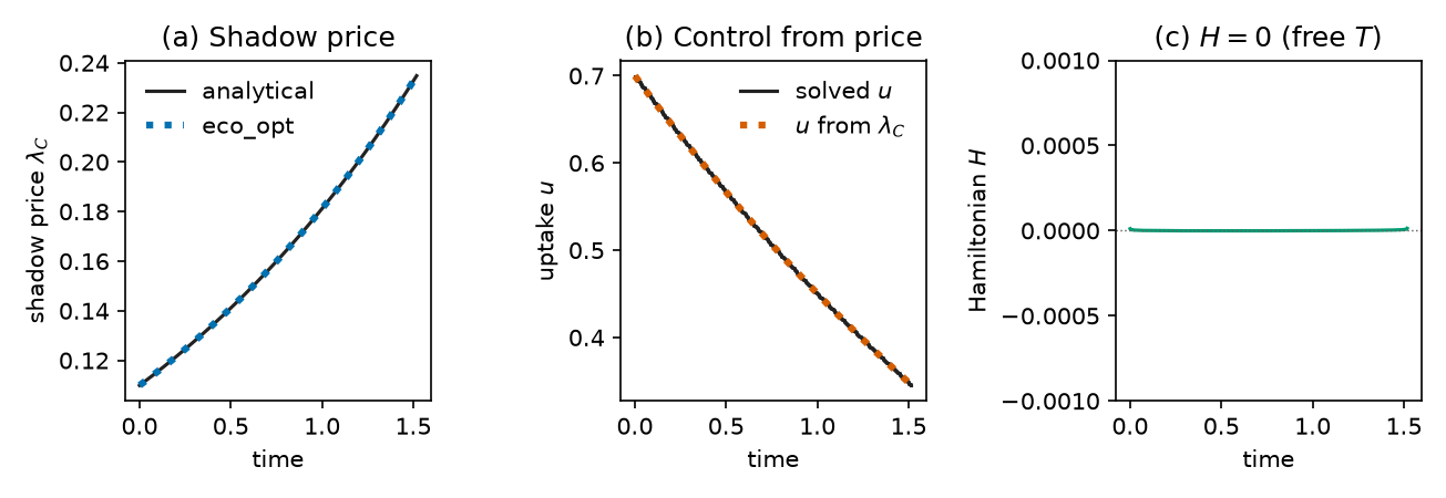
• Hamiltonian. For dynamics and running payoff without explicit time dependence, \(H\) is constant along an optimum, and \(H = 0\) when the final time is free. A drifting \(H\) signals an inaccurate solution.
• Controls that enter \(H\) linearly, such as allocation fractions. Only the sign of \(\partial H/\partial u\) matters: the control sits at its upper bound while \(\partial H/\partial u > 0\) and at its lower bound while \(\partial H/\partial u < 0\). \(\partial H/\partial u = \partial L/\partial u + \lambda^\top \partial f/\partial u\) can be evaluated from sol.costate and the model. scripts/manuscript/fig_box2_lignin.py computes \(\partial H/\partial v_O\) at \(v_O = 0\) in this way for the ligninolytic-investment model.
• Active constraints. Where a path or state constraint is active, the constraint rather than the shadow price determines the control, and the costate may jump or oscillate between collocation points.

Example: microbial uptake of a finite substrate

In the microbial-growth example, the shadow price of substrate rises as \(\lambda(t) = \lambda_T e^{\gamma (t - T)}\): substrate becomes more valuable as it runs out. The optimal uptake follows from the price, \(u = -\beta + \sqrt{e_{max}\beta(r+\beta)(\mu + 1/\lambda)}\), so a rising \(\lambda\) means slowing uptake. The figure compares the eco_opt estimate with the analytical solution of Manzoni et al. (2023).

cd examples/microbial_growth
python plot_microbial_growth.py   # writes figs/microbial_growth_costate.png

Checking them

When no analytical solution exists, check the shadow price at \(t = 0\) against a finite difference: perturb the initial state, re-solve, and compare \(\Delta J^*/\Delta x_0\) with \(\lambda(0)\). With build and optimize, only the initial-state bound changes between solves (Build and optimize).

import numpy as np
import eco_opt
from eco_opt import Namespace

BETA, GAMMA, R, EMAX, MU = 0.5, 0.5, 0.1, 0.5, 0.5


def growth_rate(u):
    return EMAX * BETA * (u - R) / (u + BETA)


def model(t, x, u):
    Cs, uptake = x[0], u[0]
    G = growth_rate(uptake)
    return -uptake - GAMMA * Cs + MU * G, Namespace(Cs=Cs, uptake=uptake)


sys = eco_opt.System(states=1, controls=1, model=model)
ocp = eco_opt.Ocp()
ocp.max([growth_rate(sys.y.uptake)])
ocp.st(
    system=sys,
    constraints=[
        (0, "==", eco_opt.t_0(sys.t)),
        (1, "==", eco_opt.t_0(sys.y.Cs)),
        (0, "<=", eco_opt.t_f(sys.t), "<=", float("inf")),
        (0, "<=", sys.y.Cs, "<=", 2),   # room above C(0) = 1 for the perturbation
        (0, "<=", sys.y.uptake, "<=", 10),
    ],
)
ocp.build(control_intervals=200, polynomial_degree=5, collocation_points="legendre")
sol = ocp.optimize(tf_guess=2.0)

# Shadow price at t = 0: extrapolate from the first two collocation points.
(t1, t2), (l1, l2) = sol.costate_time[:2], sol.costate[:2, 0]
lam0 = l1 - (l2 - l1) / (t2 - t1) * t1


def J_at(C0):
    ocp.set_constraints([(C0, "==", eco_opt.t_0(sys.y.Cs))])
    return ocp.optimize(tf_guess=2.0).objective


h = 1e-4
fd = (J_at(1 + h) - J_at(1 - h)) / (2 * h)
print(f"lambda(0) = {lam0:.5f}, finite difference = {fd:.5f}")

Expected output: lambda(0) = 0.10989, finite difference = 0.10989. The same idea checks interior times: re-solve the remaining horizon from \(x^*(t_k)\) with a perturbed state and compare with \(\lambda(t_k)\) (Bellman's principle).

tests/test_costate.py checks the costate against:

• the closed-form microbial solution, for Legendre and Radau points;
• one- and two-state linear-quadratic problems, including the Riccati solution \(\lambda = P(t)\,x(t)\) and a constant Hamiltonian;
• a problem with a terminal payoff only, where \(\lambda\) is the terminal gradient;
• finite-difference sensitivities \(\partial J^*/\partial x\) of the two-state lignin model at \(t = 0\) and at interior times.

Limitations

• Single-phase problems only.
• Accuracy follows the mesh; refine it if the costate is noisy.
• IPOPT finds local optima. A shadow price describes the optimum that was found.
• A shadow price is conditional on the model and the objective. It describes the value of a pool under the stated optimality hypothesis, not a measured property of organisms.