eco_opt

eco_opt is a Python package for turning a process-based ODE into a constrained optimal-control problem and solving it by direct collocation.

The process right-hand side is supplied by the user. Controls (quantities the modeler lets vary in time to improve \(J\)), the performance criterion, and constraints are declared. The package transcribes that statement with CasADi and solves it with IPOPT, and returns the optimal controls, the states, and the shadow prices of the states.

The modeling workflow follows Yop (Leek, 2016). eco_opt is a Python implementation of that workflow, not a copy of the Yop documentation. When an example here is a transcription of a Yop-shipped case, the example page links to the corresponding Yop page.

A complete solve

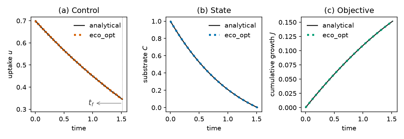
Microbial uptake of a finite substrate pulse: maximize cumulative growth while the substrate is lost at rate \(\gamma\) and partly recycled as necromass. The final time is free. Explanation: First solve.

import eco_opt
from eco_opt import Namespace

BETA, GAMMA, R, EMAX, MU = 0.5, 0.5, 0.1, 0.5, 0.5


def growth_rate(u):
    return EMAX * BETA * (u - R) / (u + BETA)


def model(t, x, u):
    Cs, uptake = x[0], u[0]
    dx = -uptake - GAMMA * Cs + MU * growth_rate(uptake)
    return dx, Namespace(Cs=Cs, uptake=uptake)


sys = eco_opt.System(states=1, controls=1, model=model)
ocp = eco_opt.Ocp()
ocp.max([growth_rate(sys.y.uptake)])
ocp.st(
    system=sys,
    constraints=[
        (0, "==", eco_opt.t_0(sys.t)),
        (1, "==", eco_opt.t_0(sys.y.Cs)),
        (0, "<=", eco_opt.t_f(sys.t), "<=", float("inf")),
        (0, "<=", sys.y.Cs, "<=", 1),
        (0, "<=", sys.y.uptake, "<=", 10),
    ],
)
sol = ocp.solve(control_intervals=200, polynomial_degree=5, tf_guess=2.0)
print(sol.success, sol.tf, sol.objective)   # True, T ~ 1.518, J ~ 0.1518

Soil and plant–soil applications

• Microbial uptake

  One state, one control, free final time. Benchmarked against the analytical solution of Manzoni et al. (2023).

• Ligninolytic investment

  Two litter pools, one control, fixed decomposition period (Chakrawal et al., 2024).

• Plant–soil C and N allocation

  Nine pools, two allocation controls, and physiological limits (Chakrawal et al., 2026).

More ecological models and textbook problems: Examples.

Start here

1. Install
2. First solve — microbial growth (finite substrate)
3. Results and plots — sol arrays and matplotlib
4. Shadow prices — marginal values of the states
5. Posing a problem — states, controls, costs
6. CasADi expressions — cs.exp, if_else, interpolants in the model
7. Transcription — piecewise-constant \(u\), collocation, mesh
8. Constraints and time — boxes, path, \(t_0\)/\(t_f\), horizon
9. Guesses, mesh, scaling — cold start, mesh, units
10. Build and optimize — frozen mesh, bound and parameter sweeps
11. Examples — ecological models, then textbook OCPs
12. Troubleshooting
13. API

What it is for

Process models in ecology are usually integrated forward: given the process equations and inputs, stocks (state variables) are predicted. Some of those inputs or rates can be treated as controls. eco_opt asks what trajectory is implied by an explicit optimality hypothesis and the same process equations, subject to constraints.

The same workflow applies to populations, water, greenhouse climate, biogeochemistry, and other process-based ecological ODEs — not only carbon allocation or organism physiology.

It does not claim that the system maximizes the chosen objective. A numerical solution shows that the hypothesis is internally consistent with the dynamics and constraints.

Cite

See Cite. Also cite CasADi, IPOPT, and Yop for the numerical stack and modeling workflow.