Quasi-steady microbes (`algebraic_qss`)¶

Question. How can fast microbial biomass be closed without a stiff biomass ODE — and why does that matter for an OCP?

Why this exists¶

Litter carbon \(C\) is slow (days to years). Microbial biomass \(M\) is fast (hours). Writing \(\dot M = \text{growth}-\text{death}\) forces tiny time steps or a stiff integrator, and in collocation it forces extra state nodes that barely move except at the start.

The quasi-steady hypothesis is: growth = death at every instant. Then \(M\) is not a differential state. It is an unknown that sits on the manifold \(g(C,M,u)=0\). The OCP still chooses uptake \(u(t)\); it just does not choose an initial \(M(0)\).

That is the value: the same optimality question (how to use a finite substrate) without pretending biomass is as slow as litter.

Formulation¶

Symbol	Role	Meaning
\(C(t)\)	differential state	substrate (slow)
\(M(t)\)	algebraic unknown	microbial biomass (fast)
\(u(t)\)	control	uptake

Differential dynamics. \(\dot C=-u\).

Algebraic closure. \(0=g(C,M,u)\) (growth = death).

Objective. \(\max\int_0^{T} M\,\mathrm{d}t\), \(T=10\) fixed.

Constraints. \(C(0)=1\), \(C\ge 0\), \(M\ge 0\), \(0\le u\le u_{\max}=0.5\). \(M\) has no initial condition.

In eco_opt: System(algebraics=1); the model returns (dx, dz, y) and dz is the residual \(g\).

Linear death (`linear_qss.py`)¶

\[ g=(e_{\max}-r u)\,u\,\frac{C}{K+C}-d M. \]

Linear in \(M\), so there is a unique formula

\[ M=\frac{(e_{\max}-r u)\,u}{d}\frac{C}{K+C}. \]

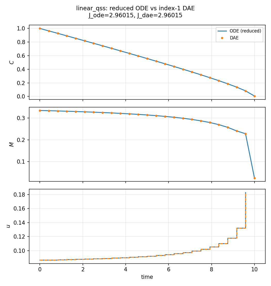
You may substitute that into \(J\) and \(\dot C\) (ordinary ODE) or keep \(M\) and \(0=g\) (DAE). Both must give the same \(J\), \(C(t)\), and \(u(t)\). That pair is the check that the algebraic transcription is not a different problem.

Quadratic death (`quadratic_qss.py`)¶

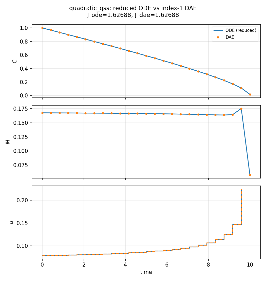
Death is \(d M + c M^2\), so \(g=0\) is a quadratic. The physical root is the plus branch of a square root; the minus root is junk. Here you do not put sqrt in \(f\): write \(0=g\) and \(M\ge 0\), and let the solver stay on the physical branch.

What was done¶

Radau collocation, degree 3. ODE vs DAE on the linear closure; DAE only on the quadratic closure.

What we found¶

Linear ODE and DAE objectives agree to about \(10^{-4}\). Trajectories of \(C\) and \(u\) overlie. The quadratic case has no explicit \(M\) and is solved only as a DAE; \(M\ge 0\) selects the physical root.

Linear QSS: ODE vs DAE

Quadratic QSS

Interpretation¶

If a pool is fast enough that you would never integrate it in a forward model (you would set growth = death and move on), it should not become a stiff ODE just because you posed an OCP. An algebraic state is that modeling choice, made visible to collocation. The linear pair (ODE vs DAE) is how you trust the implementation: same hypothesis, two writings, same \(u^*(t)\).

Public API¶

ODE vs DAE of the same hypothesis (examples/algebraic_qss/linear_qss.py):

import eco_opt
from eco_opt import Namespace


def ode_model(t, x, u):
    C, uptake = x[0], u[0]
    M = biomass(C, uptake)
    return -uptake, Namespace(C=C, M=M, u=uptake)


def dae_model(t, x, u, z):
    C, uptake, M = x[0], u[0], z[0]
    g = growth(C, uptake) - D * M
    return -uptake, g, Namespace(C=C, M=M, u=uptake)


ode = eco_opt.System(states=1, controls=1, model=ode_model)
dae = eco_opt.System(states=1, controls=1, algebraics=1, model=dae_model)

Run and tests¶

cd examples/algebraic_qss
python linear_qss.py
python quadratic_qss.py
python plot_algebraic_qss.py
python -m pytest ../../tests/test_algebraics.py -q

Quasi-steady microbes (algebraic_qss)¶