Microbial growth (microbial_growth)

Question. How should substrate uptake vary, and when should it stop, if cumulative growth is maximized while a finite resource is exhausted?

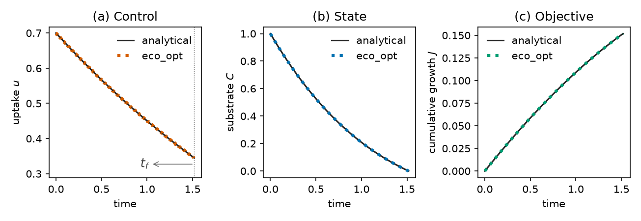
The complete first script and the eco_opt–analytical figure: First solve.

Formulation

Symbol	Role	Meaning
\(C(t)\)	state	substrate
\(u(t)\)	control	uptake rate
\(G(u)\)	diagnostic	growth rate

Dynamics.

\[ \dot C = -u - \gamma C + \mu G(u), \qquad G(u)=\frac{e_{\max}\beta(u-r)}{u+\beta}-k u. \]

Baseline: \(\beta=0.5\), \(\gamma=0.5\), \(r=0.1\), \(e_{\max}=0.5\), \(\mu=0.5\), \(k=0\). First-order decay \(\gamma\) is a parameter, not a control.

Objective.

\[ \max_{u(\cdot),\,T}\; J=\int_{0}^{T} G\bigl(u(t)\bigr)\,\mathrm{d}t. \]

Constraints.

\[ C(0)=1,\qquad 0\le C(t)\le 1,\qquad 0\le u(t)\le 10,\qquad T\ge 0. \]

Horizon. Free. The optimizer chooses when continued uptake is no longer worthwhile.

What was done

The right-hand side is the process model already used for forward simulation. Uptake is declared as u(t); \(J\) is the integral of growth; \(T\) is bounded below by zero. Direct collocation (Radau, degree 5, 200 intervals) with IPOPT.

What we found

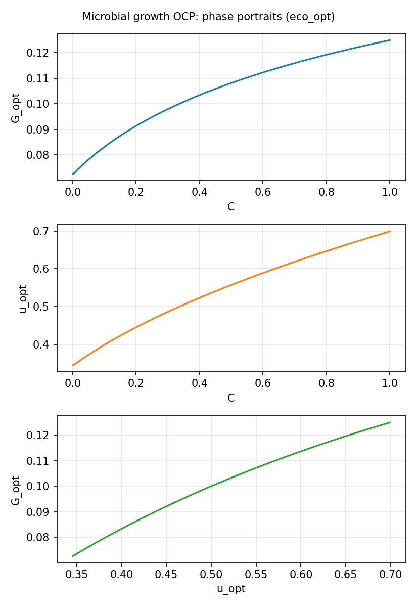
Solver succeeds; \(C(T)\to 0\) (resource exhaustion); \(C\) and \(u\) stay in their box bounds. Collocation overlays the independent analytical trajectories on First solve (\(T\approx 1.518\), \(J\approx 0.1518\)). For \(k=0\), \(r>0\), \(u^*(t)\) is a smooth interior path that declines as \(C\) is depleted.

Interpretation

A one-pool microbial model does not need a prescribed kinetic rate. An explicit growth hypothesis plus exhaustion of \(C\) already implies when uptake should fall and when activity should stop. Changing \(J\) or the bound on \(u\) would change that schedule; that is the test.

Open loop vs closed loop

An open-loop solve is a single tape \(u^*(t)\) computed from the model you wrote, then applied from \(t=0\) to \(T\) with no further looking at \(C\). That is what ocp.solve returns. Replaying it with ocp.simulate(sol) integrates the same \(\dot C=f(C,u^*)\) and must reprint \(C^*(t)\).

A closed loop (ocp.closed_loop) is different: at each sampling instant it re-solves the remaining OCP from the measured \(C\), applies only the first piece of the new \(u^*\), then waits. If the world is exactly the OCP model, the closed loop reprints the open-loop tape — there is nothing new to learn. The value appears when the simulated process is not the forecast:

• unexpected extra substrate (a pulse of \(C\) on \([0.4,0.7]\));
• a kinetic parameter that was wrong;
• a horizon that is still running after the plan assumed exhaustion.

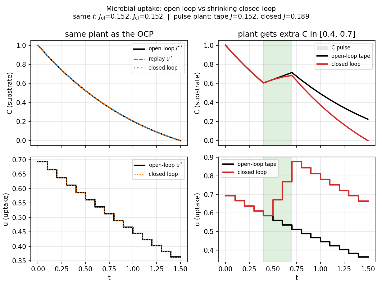
Then the tape keeps the old uptake and leaves unused \(C\). The closed loop sees the extra \(C\), raises \(u\), and captures more growth.

open_vs_closed.py pins \(T=1.5\) (the free-\(T\) optimum is about \(1.52\)) and compares those four runs. Same process: both \(u\) series match and \(\int G\approx 0.152\). Pulsed process: the tape still uses the planned uptake and leaves \(C(T)\approx 0.22\) uneaten (\(\int G\approx 0.152\)); closed loop raises \(u\) after the pulse, exhausts \(C\), and reaches \(\int G\approx 0.190\).

That gap is the reason to close the loop in a process model: the optimality hypothesis is re-evaluated on the state you actually have, not on the state you predicted on day zero.

Public API

Same solve as examples/microbial_growth/microbial_growth.py.

import eco_opt
from eco_opt import Namespace

BETA, GAMMA, R, EMAX, MU, K = 0.5, 0.5, 0.1, 0.5, 0.5, 0.0


def growth_rate(u):
    return EMAX * BETA * (u - R) / (u + BETA) - K * u


def microbial_growth_model(t, x, u):
    Cs, uptake = x[0], u[0]
    G = growth_rate(uptake)
    dx = -uptake - GAMMA * Cs + MU * G
    y = Namespace(Cs=Cs, uptake=uptake, growth=G)
    return dx, y


sys = eco_opt.System(states=1, controls=1, model=microbial_growth_model)
ocp = eco_opt.Ocp()
ocp.max([growth_rate(sys.y.uptake)])
ocp.st(
    system=sys,
    constraints=[
        (0, "==", eco_opt.t_0(sys.t)),
        (1, "==", eco_opt.t_0(sys.y.Cs)),
        (0, "<=", eco_opt.t_f(sys.t), "<=", float("inf")),
        (0, "<=", sys.y.Cs, "<=", 1),
        (0, "<=", sys.y.uptake, "<=", 10),
    ],
)
sol = ocp.solve(
    control_intervals=200,
    polynomial_degree=5,
    collocation_points="radau",
    tf_guess=2.0,
)
print(sol.success, sol.tf, sol.objective)

Run and tests

cd examples/microbial_growth
python microbial_growth.py
python plot_microbial_growth.py
python open_vs_closed.py
python -m pytest ../../tests/test_microbial_growth.py -q

References

Manzoni, Chakrawal and Ledder (2023), doi:10.3389/fevo.2023.1094269. This is not a Yop website example.