Plant–soil carbon and nitrogen (`root_opt`)¶

Question. Over a growing season, how should root carbon supply and exudation be scheduled when nitrogen can be taken up as mineral N or released by exudation-stimulated mineralisation?

Here plant means the vegetation in that coupled model.

Formulation¶

Symbol	Role	Meaning
nine C and N pools	states	leaf, root, exudate, SOM, microbial, mineral N, …
\(S(t)\)	control	root carbon supply
exudation fraction	control	share of net root assimilation that is exuded

Dynamics. Published nine-state plant–soil–microbe mass balances (leaf N diagnosed). Root growth receives what remains of root C after exudation and maintenance. Microbes take up exudate and SOM; mineralisation/immobilisation closes microbial N.

Objective.

\[ \max_{S(\cdot),\,E(\cdot)}\; J=\int_0^{T} \text{leaf growth rate}\,\mathrm{d}t, \qquad T=120\,\mathrm{d}. \]

Constraints (path). Exudation fraction in \([0.1,0.5]\); mineral-N uptake at most capacity; at least 20% of net leaf and root C to growth; non-negativity.

Horizon. Fixed growing season.

What was done¶

The published ODE is the System. Two controls replace prescribed allocation fractions. Two initial mineral-N supplies (\(20\) and \(10\,\mathrm{g\,N\,m^{-2}}\)) are compared.

What we found¶

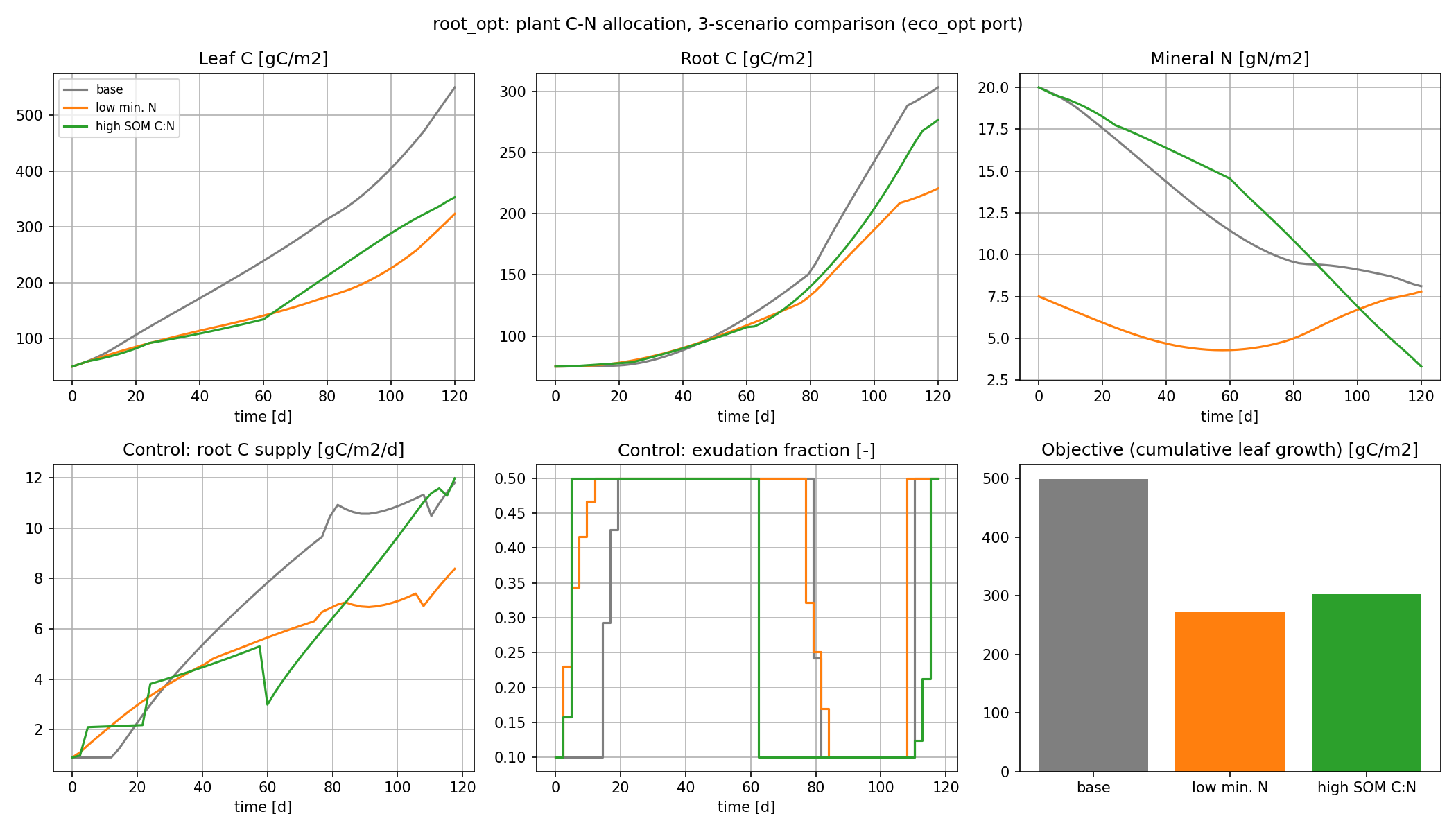
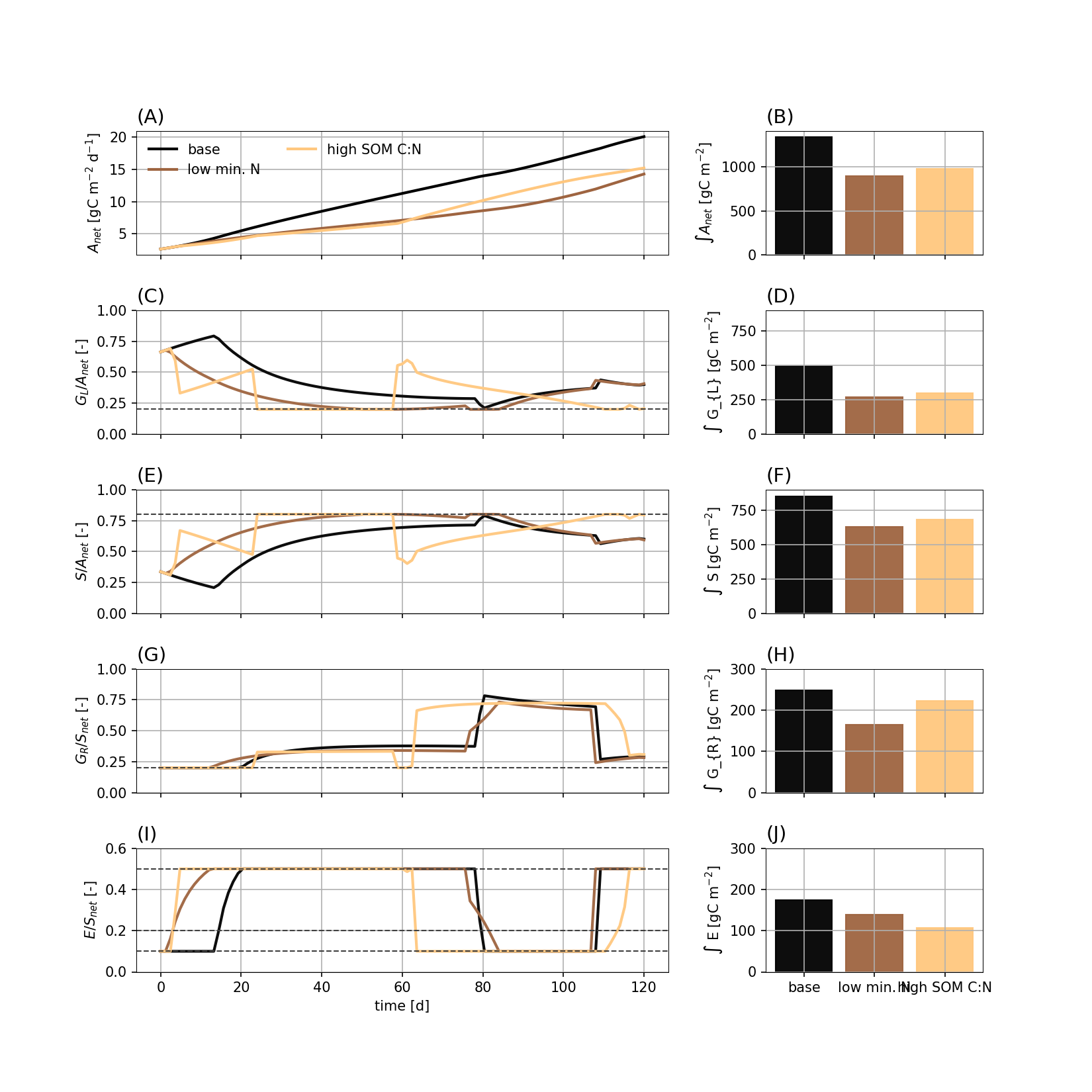
At both N supplies, exudation sits on the upper bound through mid-season, then declines as more root C goes to root growth. Lower initial mineral N raises the belowground share of net leaf assimilate and cuts leaf-C accumulation. \(J^*=499.5\,\mathrm{g\,C\,m^{-2}}\) at \(20\,\mathrm{g\,N\,m^{-2}}\) and \(322.1\) at \(10\) (control_intervals=50, degree 3).

Seasonal allocation

Published-style panels

Interpretation¶

Two belowground investments are not a single “exudation rate.” The hypothesis “maximize leaf growth over the season, with N from roots or from exudation-stimulated mineralisation” produces an early exudation phase and a later root-growth phase, and a larger belowground C commitment when mineral N is scarce. That is a schedule implied by \(J\) and the bounds, not a calibrated switch.

Open loop vs closed loop¶

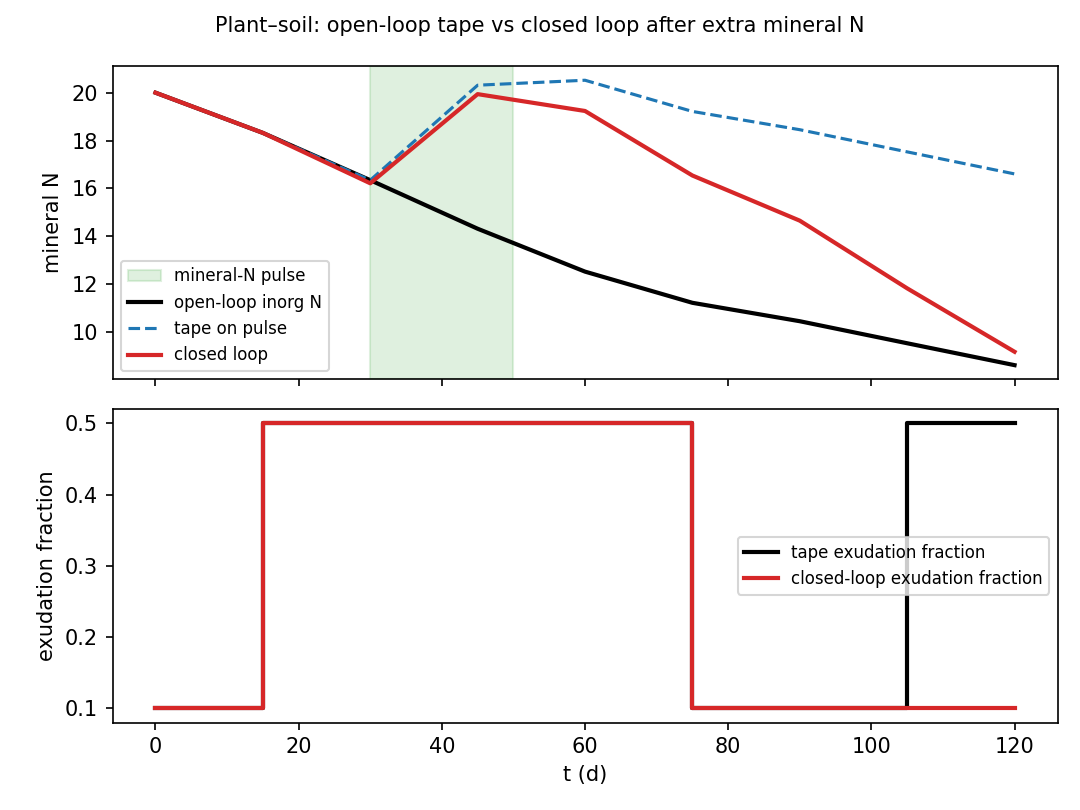
open_vs_closed.py (coarse mesh, \(N=8\)) applies the seasonal tape to a process that receives extra mineral N in days 30–50. The open-loop allocation does not see that flush. The shrinking closed loop re-solves from the measured pools, so exudation and root supply can respond. On the forecast model, closed loop should reprint the tape — the gap appears only when the soil is not the forecast.

Open vs closed loop after extra mineral N

Public API¶

Skeleton of examples/root_opt/plant_soil_nitrogen_allocation.py (nine-state RHS in that file):

import eco_opt
from eco_opt import Namespace


def plant_soil_microbe_nested(t, state, u, params=PARAMS):
    ...
    y = Namespace(leafC=fCL, leaf_growth_rate=leaf_growth, ...)
    return dx, y


sys = eco_opt.System(
    states=9,
    controls=2,
    model=lambda t, x, u: plant_soil_microbe_nested(t, x, u, PARAMS),
)
ocp = eco_opt.Ocp()
ocp.max([sys.y.leaf_growth_rate])
ocp.st(system=sys, constraints=[...])
sol = ocp.solve()

Run and tests¶

cd examples/root_opt
python plant_soil_nitrogen_allocation.py
python plot_root_opt.py
python open_vs_closed.py
python reproduce_figures.py
python -m pytest ../../tests/test_root_opt.py -q

References¶

Chakrawal, Mooney and Colombi (2026), New Phytologist doi:10.1111/nph.71210.

Plant–soil carbon and nitrogen (root_opt)¶