Lenhart and Workman labs (`lenhart_workman_labs`)¶

These examples are from Lenhart and Workman, Optimal Control Applied to Biological Models (2007).

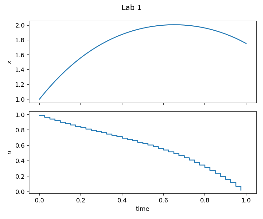
Lab 1 — Introductory example¶

Question. How does a quadratic penalty on \(u\) trade off against growing a scalar state?

Symbol	Role	Meaning
\(x\)	state	scalar stock
\(u\)	control	effort

Dynamics. \(\dot x=-\frac12 x^2+Cu\), \(x(0)=x_0>-2\).

Objective. \(\max\int_0^1(Ax-Bu^2)\,\mathrm{d}t\), \(A\ge 0\), \(B>0\).

Horizon. Fixed \(T=1\). Default \(A=B=1\), \(C=4\), \(x_0=1\).

Analytic. \(A=0\Rightarrow u^{*}\equiv 0\). Trajectories depend on \(A/B\) only. \(B=0\) and \(A>0\) has no optimum (Exercise 5.1).

Lab 1

Lab 2 — Mold and fungicide¶

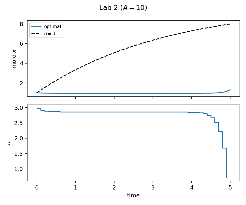
Question. Schedule fungicide to hold mold down.

Dynamics. \(\dot x=r(M-x)-ux\).

Objective. \(\min\int_0^T(Ax^2+u^2)\,\mathrm{d}t\). Default \(r=0.3\), \(M=10\), \(A=1\), \(x_0=1\), \(T=5\). Figure uses \(A=10\).

Analytic. Untreated \(x(t)=M+(x_0-M)e^{-rt}\).

Lab 2

Lab 3 — Bacteria¶

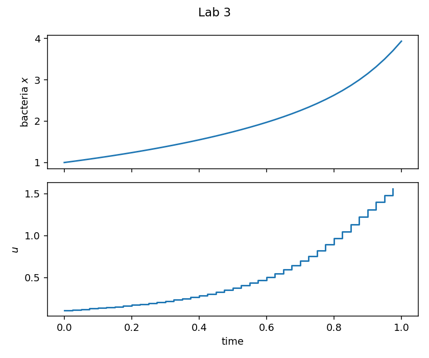
Question. Add a nutrient that also makes a harmful byproduct.

Dynamics. \(\dot x=rx+Aux-Bu^2e^{-x}\).

Objective. \(\max Cx(1)-\int_0^1 u^2\,\mathrm{d}t\) (Mayer + running). Default \(r=A=C=1\), \(B=12\), \(x_0=1\).

Analytic. \(A=0\Rightarrow u^{*}\equiv 0\); \(\lambda(1)=C\).

Lab 3

Lab 4 — Bounded case¶

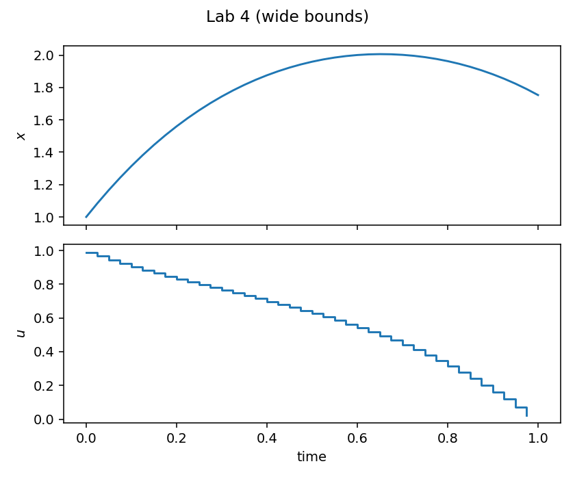
Lab 1 with \(B\) scaled out and bounds \(M_1\le u\le M_2\).

Default (9.1): \(A=1\), \(C=4\), \(x_0=1\), \(M_1=-1\), \(M_2=2\) contains the unbounded Lab 1 solution, so \(u\) is unchanged. Equal bounds \(M_1=M_2=0\) force \(u\equiv 0\).

Lab 4

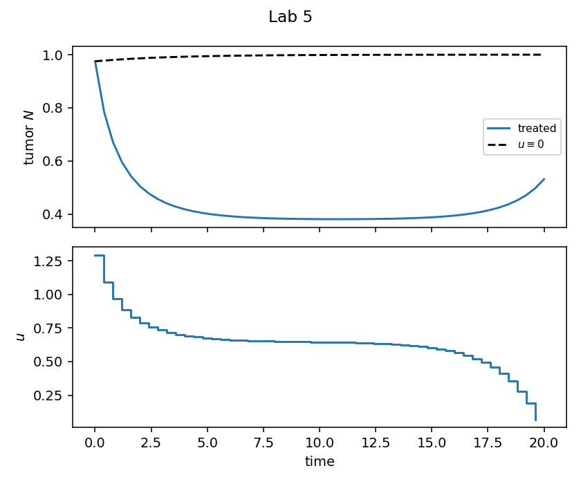
Lab 5 — Cancer¶

Skipper log-kill on Gompertz tumor density \(N\in(0,1)\).

Dynamics. \(\dot N=rN\ln(1/N)-u\delta N\), \(u\ge 0\).

Objective. \(\min\int_0^T(aN^2+u^2)\,\mathrm{d}t\). Default \(r=0.3\), \(a=3\), \(\delta=0.45\), \(N_0=0.975\), \(T=20\).

Analytic. Untreated \(N(t)=N_0^{\mathrm{e}^{-rt}}\). The bound \(u\ge 0\) is unnecessary for accepted parameters (Exercise 10.2).

Lab 5

Lab 6 — Fish harvesting¶

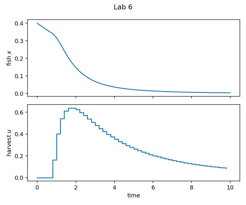
Dynamics. \(\dot x=-(m+u)x\), \(0\le u\le M\).

Objective. \(\max\int_0^T\bigl[A\frac{kt}{t+1}xu-u^2\bigr]\,\mathrm{d}t\). Default \(A=5\), \(k=10\), \(m=0.2\), \(x_0=0.4\), \(M=1\), \(T=10\).

Analytic. \(u\equiv 0\Rightarrow x=x_0e^{-mt}\). Controls depend on the product \(Ak\).

Lab 6

Lab 7 — Epidemic (SEIR vaccination)¶

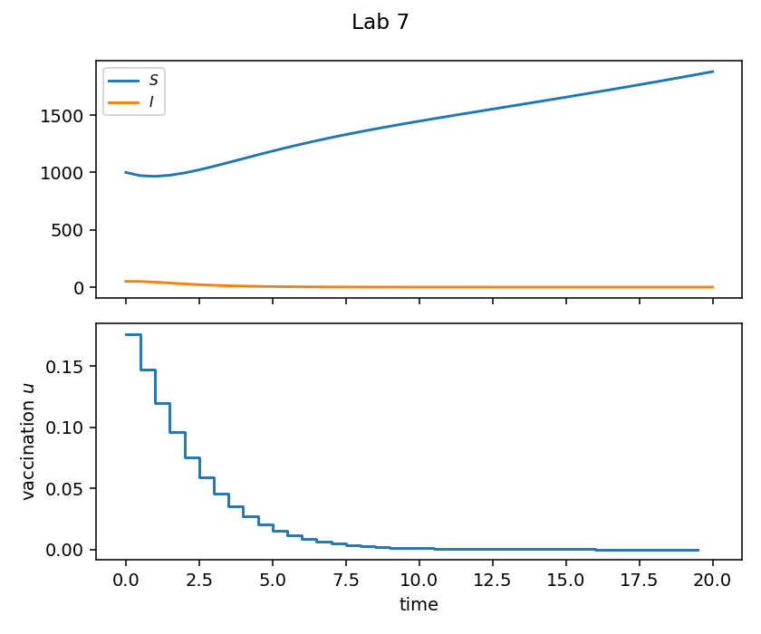
States. \(S,E,I,N\) (recovered \(R\) is not needed for the others).

Control. Fraction of susceptibles vaccinated, \(0\le u\le 0.9\).

Objective. \(\min\int_0^T(AI+u^2)\,\mathrm{d}t\). Default from the book (13.1), \(T=20\).

Lab 7

Lab 8 — HIV treatment¶

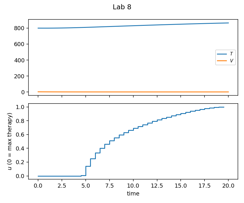
Uninfected \(T\), infected \(T_i\), virus \(V\). Control \(u=0\) is maximum reverse-transcriptase therapy, \(u=1\) is none.

Objective. \(\max\int_0^{T}[AT-(1-u)^2]\,\mathrm{d}t\). Default (14.1), \(T=20\).

Lab 8

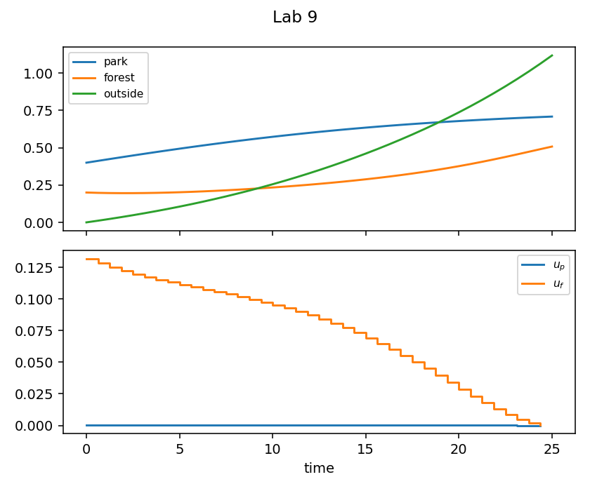
Lab 9 — Bear populations¶

Park \(P\), forest \(F\), outside \(O\); harvests \(u_p,u_f\in[0,1]\).

Objective. \(\min\int_0^T(O+c_pu_p^2+c_fu_f^2)\,\mathrm{d}t\). Default \(c_p=10^4\) so park harvest is effectively zero.

Lab 9

Lab 10 — Glucose¶

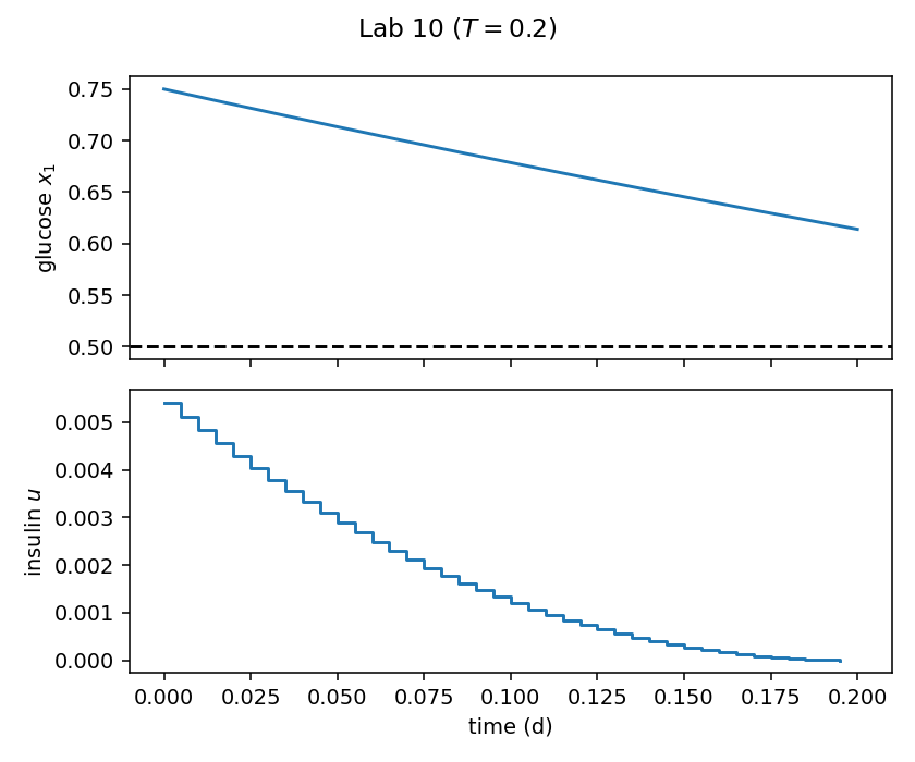
Linear glucose–hormone model with insulin \(u\).

Objective. \(\min\int_0^T\bigl[A(x_1-l)^2+u^2\bigr]\,\mathrm{d}t\). Default here is the book’s valid GTT window \(T=0.2\) (16.2), not the ill-conditioned \(T=20\) case.

Lab 10

Lab 11 — Timber harvesting¶

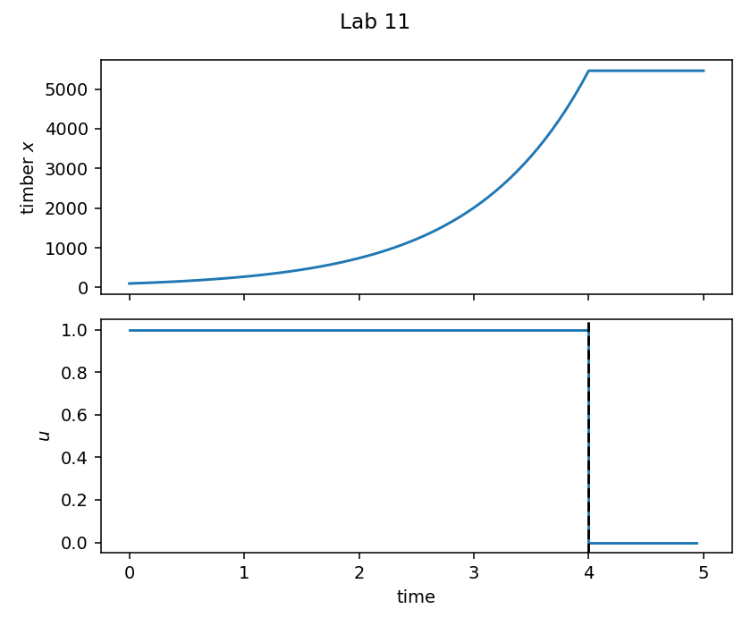
Linear in \(u\), hence bang–bang.

Dynamics. \(\dot x=kxu\), \(0\le u\le 1\).

Objective. \(\max\int_0^T e^{-rt}x(1-u)\,\mathrm{d}t\).

Analytic. No singular arc. For \(r=0\) the terminal no-investment interval has length \(1/k\), independent of \(x_0\). Default \(r=0\), \(k=1\), \(T=5\) switches at \(t^{*}=4\).

Lab 11

Lab 12 — Bioreactor¶

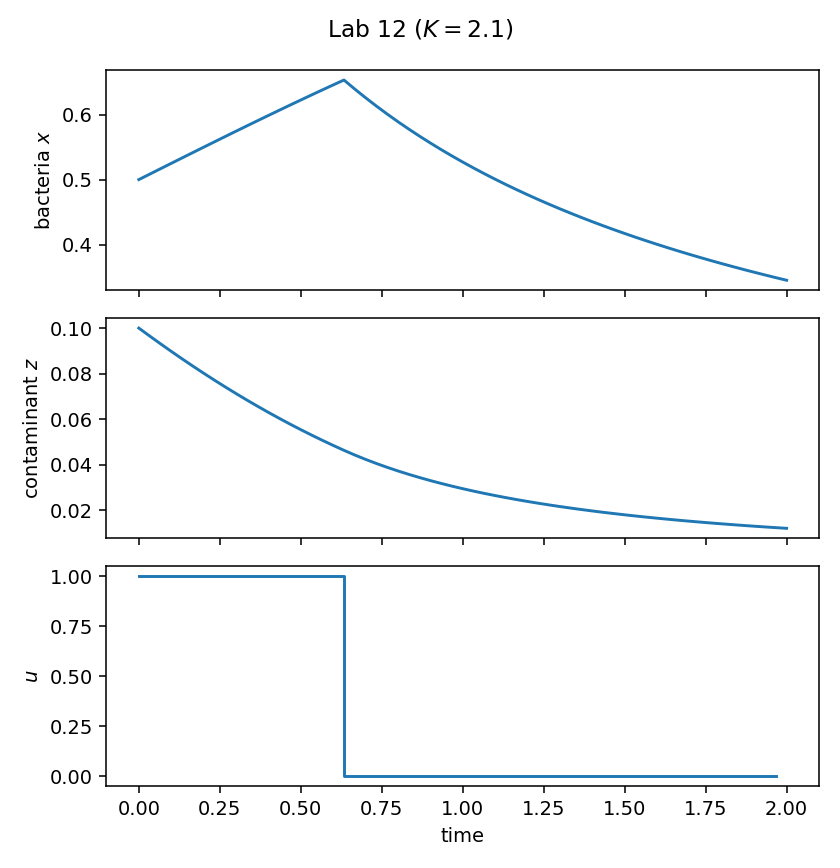
Contaminant \(z\) is eliminated: equivalent problem \(\max\int_0^T(Kx-u)\,\mathrm{d}t\), \(\dot x=Gux-Dx^2\), \(0\le u\le M\). Bang–bang. Default \(K=2\) uses no injection; \(K=2.1\) injects early. Then \(z(t)=z_0\exp(-K\int x)\).

Lab 12

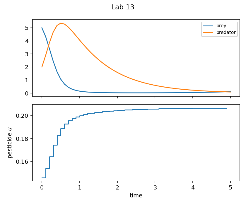
Lab 13 — Predator–prey pesticide¶

Lotka–Volterra with pesticide \(u\), box \(0\le u\le M\), and isoperimetric \(\int_0^T u\,\mathrm{d}t=B\) via an extra state \(z(0)=0\), \(z(T)=B\).

Objective. \(\min N_1(T)+\frac{A}{2}\int u^2\,\mathrm{d}t\). Default (22.2).

Lab 13

Public API¶

Each lab is import eco_opt / from eco_opt import Namespace (examples/lenhart_workman_labs/lab1_introductory.py and siblings):

import eco_opt
from eco_opt import Namespace


def lab1_model(t, x, u):
    state, ctrl = x[0], u[0]
    dx = -0.5 * state ** 2 + C * ctrl
    return dx, Namespace(x=state, u=ctrl)


sys = eco_opt.System(states=1, controls=1, model=lab1_model)
ocp = eco_opt.Ocp()
ocp.max([A * sys.y.x - B * sys.y.u ** 2])
ocp.st(system=sys, constraints=[...])

Run and tests¶

cd examples/lenhart_workman_labs
python lab1_introductory.py
python plot_labs.py
python -m pytest ../../tests/test_lenhart_workman_labs.py -q

References¶

Lenhart and Workman, Optimal Control Applied to Biological Models, Chapman & Hall/CRC, 2007.

Lenhart and Workman labs (lenhart_workman_labs)¶