Shallow lake (`shallow_lake`)¶

Question. How much phosphorus loading should be allowed, and can two long-run management strategies coexist for the same lake model?

Formulation¶

Symbol	Role	Meaning
\(P(t)\)	state	water-column phosphorus
\(L(t)\)	control	external loading (agriculture)

Dynamics.

\[ \dot P = \underbrace{L}_{\text{external loading}} - \underbrace{b P}_{\text{export / sedimentation}} + \underbrace{\frac{P^{2}}{1+P^{2}}}_{\text{internal recycling}}. \]

This is the dimensionless recycling of Mäler et al. (2003): the Hill form \(r P^{q}/(m^{q}+P^{q})\) with \(q=2\), \(m=1\), \(r=1\) (Carpenter et al. 1999). When \(P\) is small, recycling is weak. When \(P\) is large, recycling saturates near 1 and keeps the lake dirty.

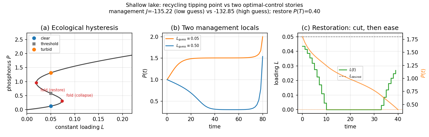
For \(b=0.52\) and constant loading in a window (\(L\approx 0.02\)–\(0.07\)) there are three equilibria: a stable clear state, an unstable threshold, and a stable turbid state. At \(L=0.05\): \(P\approx 0.13\), \(0.58\), \(1.31\).

Raising \(L\) past the upper fold collapses a clear lake to turbid. Lowering \(L\) back to the collapse value does not restore it: you must go below the lower fold (hysteresis).

Management OCP (same \(f\), loading is useful as well as harmful):

\[ \max_{L(\cdot)} \int_0^{T} e^{-\rho t} \bigl( \ln L - c P^{2} \bigr)\,\mathrm{d}t. \]

Defaults: \(b=0.52\), \(\rho=0.03\), \(c=1\), \(T=80\), \(P(0)=1\), \(10^{-3}\le L\le 1.5\).

Restoration OCP. Start turbid (\(P(0)=1.8\)), require \(P(T)\le P_{\mathrm{clean}}=0.4\), stay near a desired long-run loading \(L_{\mathrm{desired}}=0.05\):

\[ \min_{L(\cdot)}\ \int_0^{T} \bigl(L-L_{\mathrm{desired}}\bigr)^{2}\,\mathrm{d}t. \]

What was done¶

Same System; two Ocp statements. Management is solved twice from a constant high vs low guess for \(L\) (not a time-varying seed).

What we found¶

Two locals of the economic OCP, both Solve_Succeeded:

\(L_{\mathrm{guess}}\)	\(J\) (max)	\(P(T)\)
\(0.05\)	\(\approx -135.22\)	\(\approx 2.00\) (dirtier)
\(0.50\)	\(\approx -132.85\)	\(\approx 1.54\) (cleaner, better \(J\))

A true Skiba point (Skiba 1978; Wagener 2003) is an initial \(P\) where the two values are equal. Here the two \(J\)s differ, so these are two locals, one better.

Restoration: holding \(L\equiv L_{\mathrm{desired}}\) from a turbid start need not reach \(P_{\mathrm{clean}}\) (hysteresis). The solver cuts loading hard across the restore fold, then eases toward \(L_{\mathrm{desired}}\).

Hysteresis, two management locals, restoration

Interpretation¶

Two different objects share this folder. Do not conflate them.

Ecological tipping point. Lives in \(\dot P=f(P,L)\) at constant loading. Clear and turbid states, folds, hysteresis.
Two NLP locals of an OCP. Lives in the whole problem (objective
discounting + \(P(0)\) + bounds). A high vs low scalar guess for \(L\) is enough to pick which long-run lake the planner manages toward.

Initialization is part of the science here: “the solver succeeded” is not unique. The better \(J\) is the cleaner lake in this parameter set, but a cold start can still lock onto the dirtier local.

Restoration is the tipping point again: the terminal inequality \(P(T)\le P_{\mathrm{clean}}\) is not reachable by sitting at the desired loading if you start turbid.

Public API¶

Full script: examples/shallow_lake/shallow_lake.py.

import casadi as cs
import eco_opt
from eco_opt import Namespace


def lake_model(t, x, u):
    P, L = x[0], u[0]
    dP = L - B * P + P ** 2 / (1.0 + P ** 2)
    y = Namespace(P=P, L=L)
    return dP, y


sys = eco_opt.System(states=1, controls=1, model=lake_model)
ocp = eco_opt.Ocp()
ocp.max([cs.exp(-rho * sys.t) * (cs.log(sys.y.L) - c * sys.y.P ** 2)])
ocp.st(system=sys, constraints=[...])

Run and tests¶

cd examples/shallow_lake
python shallow_lake.py
python plot_shallow_lake.py
python -m pytest ../../tests/test_shallow_lake.py -q

References¶

Lake ecology: Scheffer et al. (1993); Carpenter, Ludwig and Brock (1999). OCP with two locals: Mäler, Xepapadeas and de Zeeuw (2003); Skiba (1978); Wagener (2003).

Not a figure-for-figure reproduction

The eco_opt trajectories are not validated against the numerical figures of those papers. The example follows their formulation; quantitative agreement with their plots is not claimed.

Shallow lake (shallow_lake)¶