Ligninolytic investment (opt_lignin)

Question. Over a fixed decomposition period, when should a decomposer community pay the carbon cost of oxidising aromatic litter?

Formulation

Symbol	Role	Meaning
\(C_T(t)\)	state	total remaining litter C
\(C_O(t)\)	state	aromatic (lignin-derived) C
\(v_O(t)\)	control	ligninolytic oxidation rate
\(L=C_O/C_T\)	diagnostic	aromatic fraction

Dynamics.

\[ \begin{aligned} D_H &= v_{H,\max}\,g(L)\,(C_T-C_O), \qquad D_O = v_O C_O,\\ e &= e_{\max}-r_O v_O, \qquad G = e\,(D_H+D_O),\\ \dot C_T &= -D_H-D_O+G, \qquad \dot C_O &= -D_O+\mu_O G,\\ g(L)&=\exp\bigl(-(L/a)^b\bigr). \end{aligned} \]

Growth efficiency \(e\) falls linearly with ligninolytic effort.

Objective.

\[ \max_{v_O(\cdot)}\; J=\int_0^{T} G(t)\,\mathrm{d}t. \]

Constraints. \(C_T(0)\), \(C_O(0)\) given; \(C_T\ge 0\), \(C_O\ge 0\); \(0\le v_O\le v_{O,\max}\). Horizon \(T\) fixed. Kinetic coefficients \(v_{H,\max}\), \(\mu_O\), \(r_O\) are pinned parameters.

What was done

The published process ODE is reused. \(v_O(t)\) is the only control. Kinetic coefficients are System parameters, pinned in st.

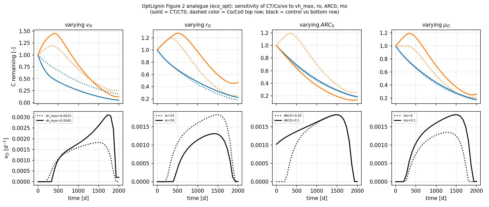
lignin_decomposition.py solves one baseline (ocp.solve, a new NLP). The \(r_O\) / \(v_{H,\max}\) / \(ARC_0\) / \(\mu_O\) sweep is plot_figure2.py: compile_ocp once, then apply_scenario → set_constraints / optimize on that mesh (Build and optimize).

What we found

Optimal \(v_O\) is near zero, then rises after a lag and later declines: hydrolytic substrate is used first. Higher \(r_O\) delays onset and lowers the peak. Baseline (\(r_O=25\,\mathrm{d}\), litter C:N 50) gives \(J^*=0.1628\).

Interpretation

A time-invariant oxidation rate hides the lag. The hypothesis “maximize growth net of oxidative cost over a fixed incubation” is enough to produce delayed ligninolysis. That lag is a prediction of the hypothesis, not an extra switch put into \(f\).

Open loop vs closed loop

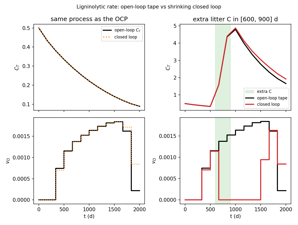
open_vs_closed.py replays \(v_O^*\) on the same litter ODE, then on a process that receives extra litter C in days 600–900. On the forecast model the shrinking closed loop reprints the tape; printed \(J=\int G\) is the realized integral along that applied \(v_O\), not ClosedLoopResults.objectives[-1] (that entry is the last remaining- horizon NLP). After the unforecast C pulse the tape keeps the old ligninolytic schedule; the closed loop re-solves from the measured \(C_T\) and can raise \(v_O\). Same lesson as microbial uptake and irrigation: the hypothesis is unchanged; the state from which it is solved is not.

Public API

Skeleton of examples/opt_lignin/lignin_decomposition.py (RHS and numeric values in that file):

import eco_opt
from eco_opt import Namespace


def lignin_model(t, x, u, p):
    CT, Co, vo = x[0], x[1], u[0]
    vh_max, mo, ro = p[0], p[1], p[2]
    ...
    y = Namespace(CT=CT, Co=Co, vo=vo, G=G)
    return dx, y


sys = eco_opt.System(states=2, controls=1, parameters=3, model=lignin_model)
ocp = eco_opt.Ocp()
ocp.max([sys.y.G])
ocp.st(system=sys, constraints=[...])
sol = ocp.solve()

Frozen-mesh sweep (plot_figure2.py):

ocp, sys = compile_ocp()
apply_scenario(ocp, sys, vh_max=..., mo=..., ro=..., ARC0=...)
sol = ocp.optimize(ipopt_options={"max_iter": 2000})

Run and tests

cd examples/opt_lignin
python lignin_decomposition.py    # baseline, ocp.solve
python plot_figure2.py            # parameter sweep, frozen mesh
python open_vs_closed.py
python -m pytest ../../tests/test_opt_lignin.py -q

References

Chakrawal et al. (2024), doi:10.1111/nph.19572.