Quickstart Guide

This guide is meant to showcase the basics of micromodel design and file exporting.

Step 1: Importing Libraries

Before starting, we will import Pore2Chip as well as some support libraries for data visualization and modification.

import pore2chip as p2c
import openpnm as op # For network visualization and for any manual topology changes
from matplotlib import pyplot as plt # For showing loaded images

Step 2: Loading Desired Data

In order to extract data from XCT images, we need to load it into memory as a 3D array of pixel values. This can be done all in one step using Pore2Chip’s built-in function read_and_filter_list. Other parameters such as cropping the image, custom threshold values, and gray value masking can also be set in the function parameters.

image_path = r'data/' # Location of the image data

# Filter and crop to 100 x 100 x 100
filtered_img_stack = p2c.filter_im.read_and_filter_list(
                                    image_path, [0, 100], [0, 100], 
                                    100, invert=True
                                )

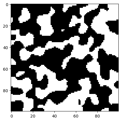
# Show the first layer using Matplotlib
fig, ax = plt.subplots()
ax.imshow(filtered_img_stack[0,:,:], cmap='gray')

Step 3: Pore Data Extraction

Now that the segmented data is loaded into memory, we will use the metrics module to extract the necessary information needed to cunstruct the micromodel design. This extraction is based on pore network extraction via watershed segmentation and the SNOW algorithm provided by Porespy.

First, we will extract the pore and pore throat diameters:

pore_diameters, throat_diameters = p2c.metrics.extract_diameters(filtered_img_stack)

Next, we will extract the pore coordination numbers:

coordination_numbers = p2c.coordination.coordination_nums_3D(filtered_images)

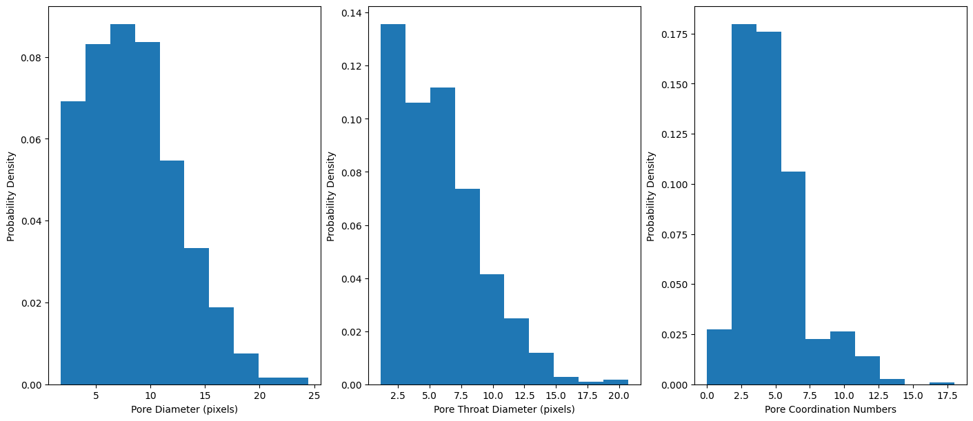
The variables we extracted are arrays that contain all of the pore diameters, throat diameters, and coordination numbers for all the extracted pores in the pore network. We can visualize the distribution of the data using matplotlib:

fig, ax = plt.subplots(1, 3, figsize=(14, 6))

ret = ax[0].hist(pore_diameters, density = True)
ret2 = ax[1].hist(throat_diameters, density = True)
ret3 = ax[2].hist(coordination_numbers, density = True)
ax[0].set_xlabel("Pore Diameter (pixels)")
ax[0].set_ylabel("Probability Density")
ax[1].set_xlabel("Pore Throat Diameter (pixels)")
ax[1].set_ylabel("Probability Density")
ax[2].set_xlabel("Pore Coordination Numbers")
ax[2].set_ylabel("Probability Density")

Note

Keep in mind that the data that is extracted is measured in the number of pixels in the segmented image. If you know the resolution size of the original XCT scan, you can scale the pixel values by the voxel size from the XCT metadata. Alternatively, you can keep note of the voxel/volume scale and adjust scaling on the final micromodel design.

Step 4: Micromodel Network Generation

Once all the necessary data is extracted (pore diameters, throat diameters, and coordination numbers), we can move on to designing the micromodel. Pore2Chip creates micromodels by constructing a 2D pore network (backed by OpenPNM) that has the overall pore properties that we extracted in step 2. Then, the network is converted from a digital representation to a shape representation using drawsvg.

To construct the 2D OpenPNM network, we will use the generate_network() function in the generate module:

network = p2c.generate.generate_network(
                                        6, 18, 
                                        pore_diameters, 
                                        throat_diameters, 
                                        coordination_numbers, 
                                        center_channel=3
                                       )

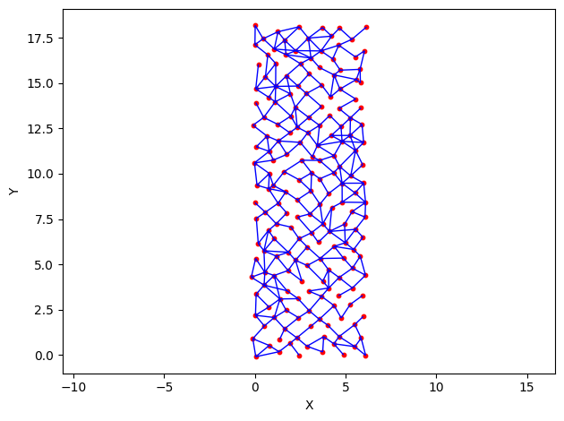
h = op.visualization.plot_connections(network)
op.visualization.plot_coordinates(network, ax=h)

The code above generates a network that is a diamond lattice of 6 x 18 pores. The generate_network() function has parameters for the number of pores on the X and Y axis, diameters, coordination numbers, and other optional arguments such as center_channel, which was used above. The argument or 3 designates a column of pores (3-wide) than the micromodel must connect from top to bottom, ensuring connectivity throughout the entire network (more info on the generation algorithm in the modules page WIP).

Step 5: Micromodel Exporting

Once we have our desired network, we will export it as a micromodel that can be used in simulations or fabrication for microfluidic experiments. This is done with the export module. We will use network2svg() to export our micromodel as a scalable vector graphic:

design = export.network2svg(network, 6, 18, 200, 600)

save_path = r'micromodel.svg' # Relative path to save file

design.save_svg(save_path) # Saves SVG file using drawsvg

This is what the exported SVG based on the OpenPNM network looks like:

This vector image can be used as is for fabrication, or imported into other software such as InkScape for further modification and exported as a DWG file compatible with most CAD software. There is also a function in export called network2dxf(), which can export a network to a DXF file that most CAD software understands, but is currently still being refined (WIP).

Note

This project is under active development.

On this page